Vegetation of East African wetlands - Assessment using R and vegtable

Example session of the work with vegetation-plot observations in R using the package vegtable and a open accessible data set of more than 300 observations collected from published references and field surveys. This tutorial explains how to use the package vegtable to process data before starting statistical assessments. An additional task handled in this document is the use of taxonomic information and further species’ attributes (traits) for calculating statistics at the plot level.

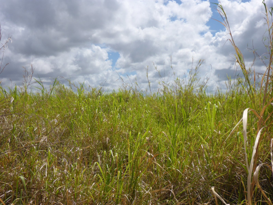
Stand of the Vigno vexillatae-Panicetum fluviicolae Behn, Alvarez, Mutebi & Becker 2022 in an undistrubed area within the Kilombero floodplain, Tanzania (CC-BY-NC K. Behn).

Introduction

This document contains an example session of the work with plot observations done in East African wetlands, mixing field surveys and data collected from published references. This data was assessed in the publication by Behn et al. (2022) and is a modified version of its Supplement S4 (Alvarez and Behn 2021).

This is an attempt to ensure reproducibility on the published statistical results and promote collaborative data assessment. Note that we use the term reproducibility in the sense of Cassey and Blackburn (2006) and Claerbout and Karrenbach (1992) but it may have a different meaning (McArthur 2019; Plesser 2018).

Required Packages

The data set is formated using the package vegtable. Taxonomic information and species attributes are embedded into vegtable but using taxlist. Furthermore, bibliographic references are included by using the package biblio.

We recommend to install all these packages from their development versions at GitHub.

library(package = "devtools")
install_github(repo = "ropensci/taxlist", build_vignettes = TRUE)
install_github(repo = "kamapu/vegtable")
install_github(repo = "kamapu/biblio")

To reproduce the interactive map at the end of this tutorial, you will need the package leaflet.

install.packages("leaflet")

Data Set

To run this session, you need to download the data by a click on this link. Then copy and paste it into your working directory.

Alternatively you may prefer to download a copy of the R-image using the following command in your running session.

download.file(url = "https://zenodo.org/record/5111485/files/swea.rda?download=1",
    destfile = "swea.rda", method = "curl")

This data set was exported from the database SWEA-Dataveg, which is registered in the Global Index of Vegetation-Plot Databases (GIVD) as AF-00-006 (Alvarez, Curran, and Malombe 2021). To optimize the content of the object, the data was pre-processed, whereby the most important changes regarding the original data are:

• Recorded sub-specific taxa (i.e. varieties and sub-species) have been merged with their respective species.
• Recorded supra-specific taxa (i.e. genera and families) have been skipped from the plot observations.
• Undetermined taxa are excluded.
• Multiple occurrence of a species in a plot have been merged preserving the maximum abundance value.
• Cover values have been equalized to the Braun-Blanquet scale for all records, where classes + and r have been merged with class 1.

To start the work with the distributed data set, you need to load vegtable to your session.

library(package = vegtable)
load(file = "swea.rda")
summary(object = swea)

## Metadata 
   name: East African Wetlands
   authors: K. Behn and M. Alvarez
   year: 2021
   object size: 419.3 Kb 
   validity: TRUE 

## Content 
   number of plots: 325 
   plots with records: 325 
   variables in header: 12 
   number of relations: 3 

## Taxonomic List 
   taxon names: 1354 
   taxon concepts: 601 
   validity: TRUE 

Taxonomic Lists

Plots observations contain records of species’ abundance in the respective plots. In vegetation-plot databases, those records may be collected from diverse sources and refer to different nomenclatures, thus a link between synonyms and accepted names to taxon concepts is required. Additionally, taxonomic ranks, parent-child relationships, and functional traits have to be considered for further ecological assessments. To deal with this, there is a slot called species including the taxonomic list in a taxlist object.

summary(object = swea@species)

object size: 244.6 Kb 
validation of 'taxlist' object: TRUE 

number of taxon usage names: 1354 
number of taxon concepts: 601 
trait entries: 320 
number of trait variables: 4 
taxon views: 6 

concepts with parents: 599 
concepts with children: 266 

hierarchical levels: form < variety < subspecies < species < genus < family < phylum 
number of concepts in level form: 0
number of concepts in level variety: 0
number of concepts in level subspecies: 0
number of concepts in level species: 335
number of concepts in level genus: 202
number of concepts in level family: 62
number of concepts in level phylum: 2

In this taxonomic list you can also query for some species using its name (partial matchings are also allowed).

summary(object = swea@species, ConceptID = "Cyclosorus interruptus",
    secundum = "bibtexkey")

------------------------------ 
concept ID: 50074 
view ID: 1 - CJBGSANBI2012 
level: species 
parent: 55055 Cyclosorus Link 

# accepted name: 
202792 Cyclosorus interruptus (Willd.) H. Itô 

# synonyms (13): 
22425 Thelypteris interrupta (Willd.) K. Iwats. 
28798 Aspidium gongylodes Schkuhr 
28802 Dryopteris gongylodes (Schkuhr) Kuntze 
28807 Pteris interrupta Willd. 
202793 Cyclosorus striatus Ching 
205463 Aspidium continuum Desv. 
205464 Aspidium ecklonii Kunze 
205465 Aspidium obtusatum Sw. 
205466 Aspidium pteroides (Retz.) Sw. 
205467 Aspidium serra (Sw.) Sw. 
205468 Aspidium serratum Sw. 
205469 Aspidium unitum (L.) Sw. 
205470 Nephrodium propinquum R. Br. 
------------------------------

This summary shows the ID of the taxon (taxon concept ID), the taxon view (reference used for the nomeclature), its taxonomic rank (level), the parent taxon (the parent genus in this case), the accepted name and a list of synonyms (both including usage name ID).

You can also use the function indented_list() to have an overview of the hierarchical structure including this taxon.

indented_list(object = swea@species, filter = "Cyclosorus")

Pteridophyta NA
 Thelypteridaceae NA
  Cyclosorus Link
   Cyclosorus interruptus (Willd.) H. Itô 

For more details on the structure of taxlist objects, see Alvarez and Luebert (2018).

Header and Relations

Information related to plot observations (e.g. soil properties, slope, exposition, coordinates) is stored as a data.frame in the slot header. In this column-oriented table the variable ReleveID represents the primary key.

head(x = swea@header)

    ReleveID original_number record_date plot_size elevation
157      259            <NA>  2012-04-25         4       348
212      249            <NA>  2012-04-18         4       351
213      246            <NA>  2012-04-18         4       333
214      245            <NA>  2012-04-18         4       343
215      250            <NA>  2012-04-18         4       351
216      221            <NA>  2012-03-27         4       337
    cover_total community_type height_total longitude  latitude
157         100            397           NA  38.32523 -5.084125
212         100            390           NA  38.32692 -5.076853
213         100            390           NA  38.32741 -5.075487
214         100            390           NA  38.32727 -5.075572
215         100            390           NA  38.32692 -5.076853
216          90            390           NA  38.32638 -5.077153
    country_code data_source
157          TZA           1
212          TZA           1
213          TZA           1
214          TZA           1
215          TZA           1
216          TZA           1

Categorical variables in header may need detailed descriptions on their respective classes, if they are factorized. For this purpose, a slot called relations contains the respective data frames. Both the data frame in the slot relations and the variable shared with slot header have the same name.

names(x = swea@relations)

[1] "community_type" "country_code"   "data_source"   

For instance the field country_code has a relation of the same name with an homonymous primary key. This field works then as a foreign key in slot header.

head(x = swea@relations$country_code)

    country_code      name_short                        name_long
17           KEN           Kenya                            Kenya
20           TZA        Tanzania                         Tanzania
33           COD Dem. Rep. Congo Democratic Republic of the Congo
38           ZAF    South Africa                     South Africa
82           ZMB          Zambia                           Zambia
125          BDI         Burundi                          Burundi

Samples

The core of plot observations is the record of taxa (usually plant species) indicating either their occurrence or their abundance in the respective plots. Since vegtable objects emulate relational databases, this information is contained in column-oriented table, at the slot samples.

head(x = swea@samples)

   ReleveID TaxonUsageID cover_percentage cover_class
15     3661          461                5           1
16     3662          461                2           1
17     3663          461                1           1
18     3748          461                1           1
19     3750          461                1           1
21     3817          461                5           1

In this table, the variable ReleveID is pointing to the plot observations in slot header, while the variable TaxonUsageID is linked to the slot species. The later is rather a mention of the taxon usage name recorded in the plot, which will be recognized either as synonym or accepted name of a taxon concept. The abundance of the species in plots (variable cover_class) corresponds to the Braun-Blanquet scale with the classes “+” and “r” merged with “1”, as previously mentioned.

Cocktail Classification

Cocktail classification is a supervised classification method based on logical algorithms. The main elements in these algorithms are the definition of species groups (cocktail groups) and dominant species. The algorithms will recognize plot observations in a vegetation unit by the occurrence of more than a half of the members of a coctail group, the absence of a group and whether a dominant species is present over a cut-level of abundance or not (Bruelheide 1997; Kočı́, Chytrý, and Tichý 2003).

The package vegtable defines an object class called shaker. This object will always depend on a vegtable object (companion). A shaker is included in the distributed image, which is called syntax.

summary(object = syntax, companion = swea)

The design of cocktail algorithms is a time-consuming, iterative process and will not be explained here. We recommend to use the software Juice for this purpose (Tichý 2002). The function make_cocktail() will execute the expert system and produce the classification that can be inserted in the data set.

swea@header <- make_cocktail(shaker = syntax, vegtable = swea, cover = "cover_class",
    syntax = "veg_unit")

For every formula contained in syntax, a binary variable indicating whether a plot is belonging to a vegetation unit or not. Additionally a column defined as veg_unit is inserted with the name of the respective units. Note that in this column observations that are not recognized in any vegetation unit get a NA value, while observation recognized in more than one unit get a + symbol.

summary(object = as.factor(x = swea$veg_unit))

        + 01Isc-Fim 02Fui-Amm 03Cor-Pan 04Gra-Ipo 05Cen-Per 06Cyp-Cyp 
       36        11         8        17         8        12        59 
07Cyp-Fui 08Mel-Lee 09Cyp-lat 10Cyp-Dry 11Phr-mau  12PhrEch 13Vig-Pan 
       42        19        25        50        22         5        11 

Statistics from Taxon Traits

Life Forms and Origin

The taxonomic list includes information on life forms and origin (native or introduced to sub-Saharan Africa). This information can be summarized for every plot, for instance calculating the proportion of life forms, weighted by the abundance. For it, we can use the function trait_proportion(), which will aggregate proportions of single life form classes into plot observations. Since we like to collect the information in the slot header with further plot properties, we will use the option in_header=TRUE.

swea <- trait_proportion(trait = "life_form", object = swea, weight = "cover_class",
    in_header = TRUE)

# Boxplot
par(las = 1, mar = c(4, 8, 1, 1))
boxplot(formula = obligate_annual_prop ~ veg_unit, data = swea@header, horizontal = TRUE,
    col = "grey", ylab = "", xlab = "Proportion of Annual Plants")
abline(v = 0.5, lty = "dashed")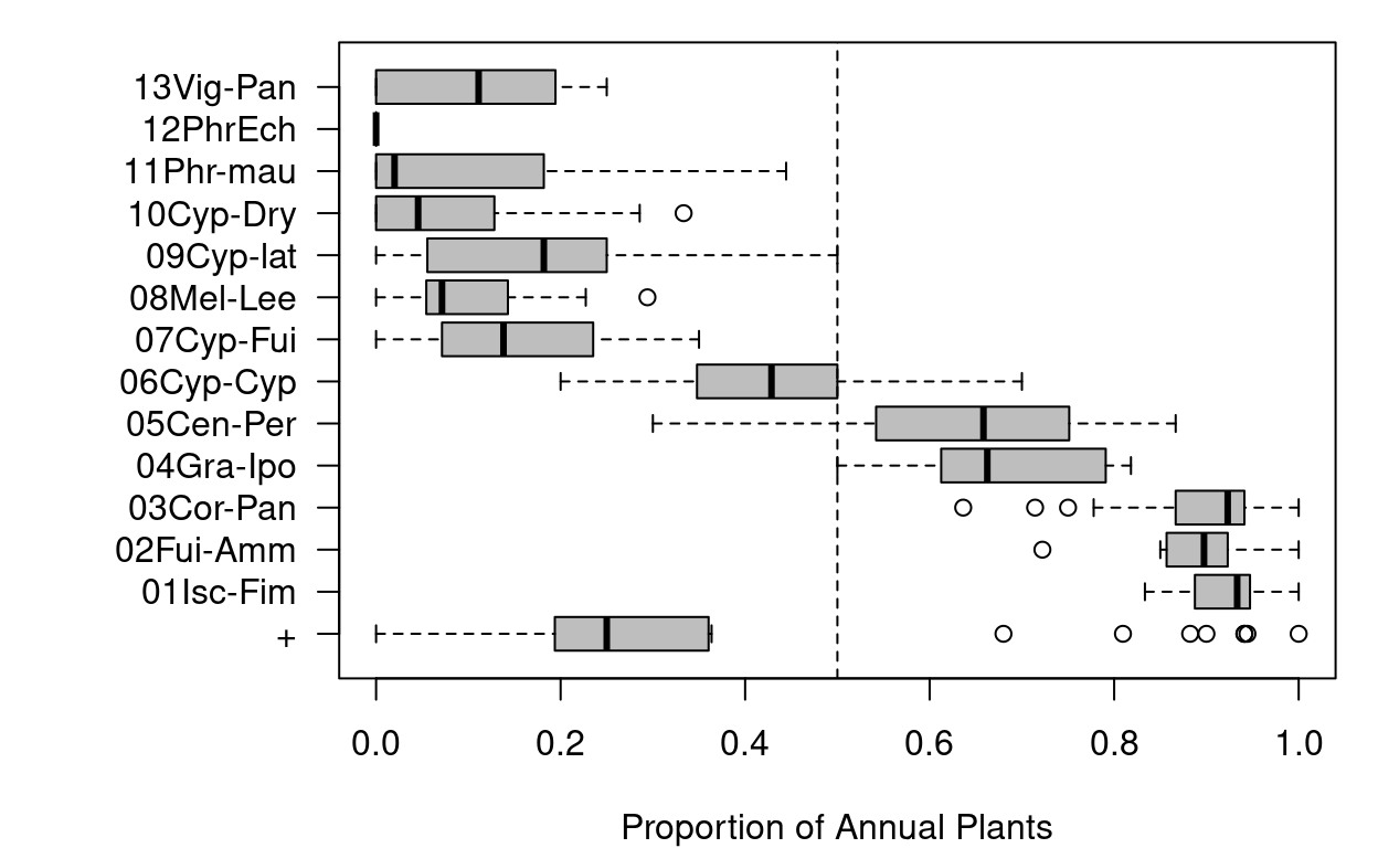

Note that trait_proprotion() is designed to calculate proportions of categorical traits. Alternatively the function trait_stats() is suitable for statistics of numerical traits (e.g. calculation of weighted averages).

Taxonomy

Taxonomic information is not mandatory in taxonomic lists. In slot species of the object swea both, the taxonomic ranks and the parent-child relationships are included.

summary(object = swea@species)

object size: 244.6 Kb 
validation of 'taxlist' object: TRUE 

number of taxon usage names: 1354 
number of taxon concepts: 601 
trait entries: 320 
number of trait variables: 4 
taxon views: 6 

concepts with parents: 599 
concepts with children: 266 

hierarchical levels: form < variety < subspecies < species < genus < family < phylum 
number of concepts in level form: 0
number of concepts in level variety: 0
number of concepts in level subspecies: 0
number of concepts in level species: 335
number of concepts in level genus: 202
number of concepts in level family: 62
number of concepts in level phylum: 2

For statistical assessments it is necessary to set taxonomic information as species traits. This can be managed with the function tax2traits().

swea@species <- tax2traits(object = swea@species, get_names = TRUE)
head(x = swea@species@taxonTraits)

   TaxonConceptID     life_form origin_ssa origin_source
2           56944 tussock_plant     native             3
4           56931 tussock_plant     native             3
6           56768 tussock_plant     native             3
8             249 tussock_plant     native             3
9           54697 tussock_plant     native             3
10          52150  annual_plant  adventive             3
                  origin_remarks                 species     genus
2                           <NA>    Anosporum pectinatum Anosporum
4                           <NA>            Carex mannii     Carex
6                           <NA>     Cyperus platycaulis   Cyperus
8                           <NA>      Epilobium salignum Epilobium
9                           <NA> Epilobium stereophyllum Epilobium
10 Mexico to S. Tropical America    Erigeron sumatrensis  Erigeron
       family        phylum
2  Cyperaceae Magnoliophyta
4  Cyperaceae Magnoliophyta
6  Cyperaceae Magnoliophyta
8  Onagraceae Magnoliophyta
9  Onagraceae Magnoliophyta
10 Compositae Magnoliophyta

The last function inserted new columns for taxonomic ranks indicating the usage name of each taxon (without author name) and its respective parent taxa. In the next step we will calculate the frequency of species in each family.

# Counting species per family
Families <- count_taxa(object = species ~ family, data = swea@species)

# Sorting families by frequency
Families <- Families[order(Families$species_count, decreasing = TRUE), ]

# Ploting the 20 most frequent families
par(las = 2, mar = c(10, 5, 1, 1))
with(data = Families[1:20,], expr = barplot(species_count, names.arg = family,
        ylab = "Number of Species"))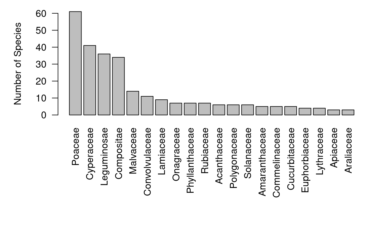

To see if there is some trend in the proportion of a family, for instance Poaceae, we can use again the function trait_proportion(). Herewith we will weight the proportion of families by the abundance of the respective species in the plot.

swea <- trait_proportion(trait = "family", object = swea, weight = "cover_class",
    in_header = TRUE)

# Boxplot
par(las = 1, mar = c(4, 8, 1, 1))
boxplot(formula = Poaceae_prop ~ veg_unit, data = swea@header, horizontal = TRUE,
    col = "grey", ylab = "", xlab = "Proportion of Grasses")
abline(v = 0.5, lty = "dashed")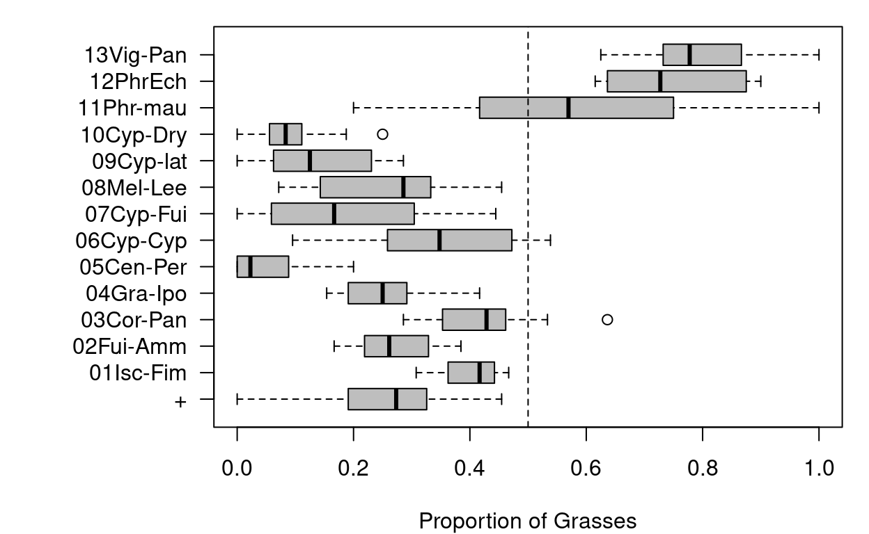

Export Functions

The structure of vegtable objects is quite complex and some assessments or displays will require a proper export method. Here we introduce some of the basic ways to export information for further assessments. For instance, some of those functions will work on a subset of plots, which include the species Cyperus papyrus L.

cype_pap <- subset(x = swea, subset = TaxonName == "Cyperus papyrus", slot = "taxonNames")

In the previous step only records for C. papyrus L. are preserved, thus we will use the plot observation ids to produce a subset with full relevés.

cype_pap <- subset(x = swea, subset = ReleveID %in% cype_pap$ReleveID, slot = "header")

Cross-table

The most common format for displaying vegetation data is the cross table, with species as rows and plots as columns. To produce cross tables there is the function crosstable(). This function requires a formula in the form abundance twidles species and plot (in the example, cover_class ~ ReleveID + AcceptedName) and a function to summarize multiple occurrences of a species in a plot (e.g. the maximum value). Depending on the size of the data set, this process may require some seconds.

Table <- crosstable(formula = cover_class ~ ReleveID + AcceptedName, data = cype_pap,
    FUN = max)

Note that the terms ReleveID and AcceptedName are the key variables for the slot header and the object taxlist in slot species, respectively.

It is also possible to insert additional columns besides the species list, for instance to add the author name (AuthorName in taxlist) and the family, you need to add them as terms in the formula.

Table <- crosstable(formula = cover_class ~ ReleveID + AcceptedName + AuthorName + family,
    data = cype_pap, FUN = max, na_to_zero = TRUE)

# First 5 rows and 10 columns
Table[1:5, 1:10]

           AcceptedName                     AuthorName      family
1   Asystasia gangetica               (L.) T. Anderson Acanthaceae
2 Hygrophila auriculata              (Schumach.) Heine Acanthaceae
3    Hypoestes aristata (Vahl) Sol. ex Roem. & Schult. Acanthaceae
4      Thunbergia alata                  Bojer ex Sims Acanthaceae
5 Acanthus polystachyus                         Delile Acanthaceae
  3698 3739 3882 4752 4945 4950 5256
1    1    1    1    1    1    1    1
2    0    0    0    0    0    0    0
3    0    0    0    0    0    0    4
4    0    0    0    0    0    0    0
5    0    0    1    0    0    0    0

Some statistical software and R-packages may need the first cross table but transposed. This can be achieved by changing the formula in the function.

Table <- crosstable(formula = cover_class ~ AcceptedName + ReleveID, data = swea,
    FUN = max, as_matrix = TRUE)

Juice table

There is also a possibility to export the content of plot observations to Juice. Juice is a freeware specialized in the analysis of vegetation-plot data sets and implement a series of statistical assessment methods. To produce the data sets, there is the function write_juice(), which is working in a similar way as crosstable(). Here we need additionally to specify which header variables will be exported and which are the geographical coordinates (assumed as decimal degrees in WGS84).

write_juice(data = swea, file = "swea", formula = cover_class ~ ReleveID + AcceptedName, 
    db_name = swea@description$name,
    header = c("country_code", "data_source", "record_date", "plot_size", "elevation",
        "veg_unit"),
    coords = c("longitude", "latitude"), FUN = max)

This command will produce two files in your working directory, the file swea_table.txt with the cross table, and swea_header.txt with the information of plots (also called header table). To import those files to Juice, yo need to follow these steps.

Map

The plot observations included in this data set are geo-referenced, where the exactitude of the location is depending on the data source (some data are geo-referenced according to the study site description of the respective publication).

The location of plot observations can be mapped by using the package leaflet.

library(package = leaflet)
leaflet(data = swea@header, width = "100%") %>%
    addProviderTiles("Esri.WorldImagery") %>%
  addMarkers(lng = ~longitude, lat = ~latitude, popup = ~paste(ReleveID),
      clusterOptions = markerClusterOptions()) %>%
    addMiniMap(width = 100, height = 100)

Updated on

31-07-2022