The program of the workshop is accessible here.
First Steps
This session deals with the management and process of taxonomic lists and retrieving information from vegetation-plot databases. Following software will be required for this session:
Installation of requirements in R
Though all required R-packages will be installed in the computer room
previous to this session, here there are instructions, in the case you
try to repeat the sessions in your own computer. Following command line
should be executed in order to install all required packages in
R:
install.packages(c("devtools", "foreign", "plotKML", "rgdal", "sp", "vegdata",
  "vegan", "xlsx"), dependencies=TRUE)
This session will focus on the use of two packages that use GitHub as repository for
sharing and development. The package taxlist
processes taxonomic lists that may be connected to biodiversity
information (e.g. vegetation relevés), while the package vegtable has
a similar task but handling vegetation-plot records. Since
vegtable is depending on taxlist, both
packages should be installed and updated for this session:
library(remotes)
install_github("ropensci/taxlist", build_vignettes=TRUE)
install_github("kamapu/vegtable", build_vignettes=TRUE)
Since both package are been uploaded in the Comprehensive R Archive Network (CRAN), you can also use the common way to get the last released version.
install.packages("vegtable", dependencies=TRUE)
Documents and data sets
This is the main document of the Workshop and will be distributed
among its participants. Additionally, data sets required for the
examples are provided by the installation of the R-packages
taxlist and vegtable.
Introduction to taxlist
The package taxlist define an homonymous S4
class. Among other properties, S4 classes implement a
formal definition of objects, tests for their validation and functions
(methods) applied to them. Such properties are suitable for structure
information of taxonomic lists and for data handling.
This class is composed by four slots, corresponding to
column-oriented tables (class data.frame in
R). While the slots taxonNames and
taxonRelations contain the information on names (labels of
taxon concepts) and taxon concepts, respectively, representing the core
information of taxonomic lists.
most important information regarding taxa (taxon concepts),
information in slots taxonTraits and
taxonViews is optional and they can be empty.
Building taxlist objects
Building taxlist objects can be achieved either through
a step-by-step routine working with small building blocks or by
importing consolidated data sets.
Using character vectors
Objects of class taxlist can be just built from a list
of names formatted as a character vector. To achieve it, the functions
new and add_concept are required.
plants <- c("Lactuca sativa","Solanum tuberosum","Triticum sativum")
splist <- new("taxlist")
splist <- add_concept(splist, plants)
summary(splist)
Using formatted tables
In the case of consolidated species lists, they can be inserted in a
table previously formatted for taxlist (or
Turboveg). Such tables can include both, accepted names
for plant species as well as their respective synonyms. A formatted
table is installed in the package taxlist.
File <- file.path(path.package("taxlist"), "cyperus", "names.csv")
Cyperus <- read.csv(File, stringsAsFactors=FALSE)
str(Cyperus)
This table was originally imported form Turboveg and
inherits some of its default columns. Four columns were renamed and are
mandatory for process the table with the function
df2taxlist:
TaxonUsageIDis the key field of a table of names (slottaxonNames).TaxonConceptIDis the link of the name to its respective concept (key field in slottaxonRelations.TaxonNameis the name itself as character.AuthorNameis a character value indicating the author(s) of the respective name.
Additionally the functions require a logical vector indicating, which
of those names should be considered as synonyms or accepted names for
its respective concept. This information is provided by the inverse
value of the column SYNONYM in
Turboveg.
Cyperus <- df2taxlist(Cyperus, !Cyperus$SYNONYM)
summary(Cyperus)
object size: 32.1 Kb
validation of 'taxlist' object: TRUE

number of taxon usage names: 95
number of taxon concepts: 42
trait entries: 0
number of trait variables: 0
taxon views: 0
Using Turboveg species list
A direct import from a Turboveg database can be done
using the function tv2taxlist. The installation of
vegtable includes data published by Fujiwara et
al. (2014) with vegetation plots collected in forest stands
from Kenya.
library(vegtable)
tv_home <- file.path(path.package("vegtable"), "tv_data")
Fujiwara <- tv2taxlist("Fujiwara_sp", tv_home)
summary(Fujiwara)
Summary displays
For taxlist objects there are basically two ways for
displaying summaries. The first way is just ot apply the function
summary to a taxlist object:
summary(Cyperus)
object size: 32.1 Kb
validation of 'taxlist' object: TRUE

number of taxon usage names: 95
number of taxon concepts: 42
trait entries: 0
number of trait variables: 0
taxon views: 0
Note that this option also executes a validity check of the object,
as done by the function validObject.
The second way is getting information on a particular concept by adding it concept ID or a taxon usage name as second argument in the function.
summary(Cyperus, "Cyperus dives")
------------------------------
concept ID: 197
view ID: none
level: none
parent: none

# accepted name:
197 Cyperus dives Delile

# synonyms (5):
52000 Cyperus immensus C.B. Clarke
52600 Cyperus exaltatus var. dives (Delile) C.B. Clarke
52601 Cyperus alopecuroides var. dives Boeckeler
52602 Cyperus immensus var. petherickii (C.B. Clarke) Kük.
52603 Cyperus petherickii C.B. Clarke
------------------------------
Specific information for several concepts can be displayed by using a
vector with several concept IDs. Through the option
ConceptID="all" it is also possible to get a display of the
first concepts, depending on the value of the argument
maxsum.
summary(Cyperus, "all", maxsum=10)
Example data set
The installation of taxlist includes the data
Easplist, which is formatted as a taxlist
object. This data is a subset of the species list used by the database
SWEA-Dataveg (GIVD ID
AF-006):
Access to slots
The common ways to access to the content of slots in S4
objects are either using the function slot(object, name) or
the symbol @ (i.e. object@name). Additional
functions, which are specific for taxlist objects are
taxon_names, taxon_relations,
taxon_traits and taxon_views (see the help
documentation).
Additionally, it is possible to use the methods $ and
[ , the first for access to information in the slot
taxonTraits, while the second can be also used for other
slots in the object.
  acropleustophyte        chamaephyte     climbing_plant facultative_annual
                 8                 25                 25                 20
   obligate_annual       phanerophyte   pleustohelophyte         reed_plant
               114                 26                  8                 14
     reptant_plant      tussock_plant               NA's
                19                 52               3576
Subsets
Methods for the function subset are implemented in order
to generate subsets of the content of taxlist objects. Such
subsets usually apply pattern matching (for character vectors) or
logical operations and are analogous to query building in relational
databases. The subset method can be apply to any slot by
setting the value of the argument slot.
Or the very same results:
Similarly, you can look for a specific name.
Parent-child relationships
Objects belonging to the class taxlist can optionally
content parent-child relationships and taxonomic levels. Such
information is also included in the data Easplist, as shown
in the summary output.
summary(Easplist)
object size: 761.4 Kb
validation of 'taxlist' object: TRUE

number of taxon usage names: 5393
number of taxon concepts: 3887
trait entries: 311
number of trait variables: 1
taxon views: 3

concepts with parents: 3698
concepts with children: 1343

hierarchical levels: form < variety < subspecies < species < complex < genus < family
number of concepts in level form: 2
number of concepts in level variety: 95
number of concepts in level subspecies: 71
number of concepts in level species: 2521
number of concepts in level complex: 1
number of concepts in level genus: 1011
number of concepts in level family: 186
Note that such information can get lost once applied
subset, since the respective parents or children from the
original data set are not anymore in the subset. May you like to recover
parents and children, you can use the functions get_paretns
or get_children, respectively.
summary(Papyrus, "all")
------------------------------
concept ID: 206
view ID: 1
level: species
parent: none

# accepted name:
206 Cyperus papyrus L.

# synonyms (2):
52612 Cyperus papyrus ssp. antiquorum (Willd.) Chiov.
52613 Cyperus papyrus ssp. nyassicus Chiov.
------------------------------
Papyrus <- get_parents(Easplist, Papyrus)
summary(Papyrus, "all")
------------------------------
concept ID: 206
view ID: 1
level: species
parent: 54853 Cyperus L.

# accepted name:
206 Cyperus papyrus L.

# synonyms (2):
52612 Cyperus papyrus ssp. antiquorum (Willd.) Chiov.
52613 Cyperus papyrus ssp. nyassicus Chiov.
------------------------------
concept ID: 54853
view ID: 2
level: genus
parent: 55959 Cyperaceae Juss.

# accepted name:
54855 Cyperus L.
------------------------------
concept ID: 55959
view ID: 3
level: family
parent: none

# accepted name:
55961 Cyperaceae Juss.
------------------------------
Introduction to vegtable
Objects of class vegtable are complex objects attempting
to handle the most important information contained in vegetation-plot
databases. They are defined in the homonymous package, while the species
list will be required as a taxlist object.
As already mentioned, S4 objects are composed by
slots:
The information contained in the slot is the following:
descriptionis containing the “metadata” of the database as a named character vector.samplesis a column oriented table with the observations of species (as usage IDs) in plots and layers.headeris a table containing information on the plots.speciesis the taxonmic list astaxlistobject.relationsare tables linked to categorical variables in slotheader(calledpopupsin Turboveg).coverconvertis a list with conversion tables among cover scales.
Building vegtable objects
An empty object (prototype) can be generated by using the function
new:
Veg <- new("vegtable")
It is also possible to build an object from cross tables, assuming all species included in the table are accepted names:
File <- file.path(path.package("vegtable"), "Fujiwara_2014", "samples.csv")
Fujiwara <- read.csv(File, check.names=FALSE, stringsAsFactors=FALSE)
Fujiwara_veg <-df2vegtable(Fujiwara, 1, 2)
summary(Fujiwara_veg)
Example data set
The package vegtable also provides own data sets as
examples. One of those examples is dune_veg, which contains
the data sets dune and dune.env from the
package vegan.
Other example is Kenya_veg, which also represent a
subset of the database SWEA-Dataveg (GIVD ID
AF-00-006).
## Metadata
   db_name: Sweadataveg
   sp_list: Easplist
   dictionary: Swea
   object size: 9501 Kb
   validity: TRUE

## Content
   number of plots: 1946
   plots with records: 1946
   variables in header: 34
   number of relations: 3

## Taxonomic List
   taxon names: 3164
   taxon concepts: 2392
   validity: TRUE
As shown in the previous commands, the function summary
displays a general overview of the object’s content, while it also runs
a validity check. An additional display is offered by the function
vegtable_stat:
vegtable_stat(Kenya_veg)
## Metadata
   db_name: Sweadataveg
   sp_list: Easplist
   dictionary: Swea
   object size: 9501 Kb
   validity: TRUE

## Content
   number of plots: 1946
   plots with records: 1946
   variables in header: 34
   number of relations: 3

## Taxonomic List
   taxon names: 3164
   taxon concepts: 2392
   validity: TRUE

REFERENCES
Primary references: 5

## AREA
Area range (m^2): 150 - 1750
<1 m^2: 0%
1-<10 m^2: 0%
10-<100 m^2: 0%
100-<1000 m^2: 2%
1000-<10000 m^2: 1%
>=10000 m^2: 0%
unknow: 97%

## TIME
oldest: 1983 - youngest: 2014
<=1919: 0%
1920-1929: 0%
1930-1939: 0%
1940-1949: 0%
1950-1959: 0%
1960-1969: 0%
1970-1979: 0%
1980-1989: 36%
1990-1999: 31%
2000-2009: 2%
2010-2019: 1%
unknow: 30%

## DISTRIBUTION
KE: 100%

## PERFORMANCE
01: 83%
02: 17%
03: 0%
04: 0%
05: 0%
06: 0%
07: 0%
08: 0%
09: 0%
10: 0%
11: 0%
12: 0%
Access to slots
Some functions are provided for the access to slots of
vegtable objects, namely header and
veg_relation, taxon_traits and
taxon_views (see the help documentation).
For a direct access of the content included in slot
header, there are the methods $ and
[:
summary(Kenya_veg$REFERENCE)
veg_relation(Kenya_veg, "REFERENCE")[,1:3]
Subsets
As a way to generate queries from vegtable objects, a
method for the function subset is implemented as well.
Following is the case of the data set dune_veg generating a
subset with pasture plots.
## Metadata
   object size: 22.2 Kb
   validity: TRUE

## Content
   number of plots: 20
   plots with records: 20
   variables in header: 6
   number of relations: 0

## Taxonomic List
   taxon names: 30
   taxon concepts: 30
validity: TRUE summary(pasture)
## Metadata
   object size: 19.4 Kb
   validity: TRUE

## Content
   number of plots: 5
   plots with records: 5
   variables in header: 6
   number of relations: 0

## Taxonomic List
   taxon names: 30
   taxon concepts: 30
   validity: TRUE
Cross tables
Most of the applications dealing with analysis of vegetation tables
(e.g. the package vegan) will deal with cross tables rather
than with column-oriented database lists. Therefore a function
crosstable is defined for the conversion of
taxlist objects to cross tables. Before building a cross
table it will be recommended to transform the cover into percentage
value by using the function transform.
pasture <- cover_trans(pasture, to="Cover", rule="middle")

Cross <- crosstable(Cover ~ ReleveID + AcceptedName, pasture, max,
  na_to_zero=TRUE)
Cross
The first argument in the function is the formula
y ~ x1 + x2 + ... + xn, where:
yis the cover value (a column in slotsamples).x1is the plot ID or a grouping value from slotheaderwhich will be used as columns in the cross table.x2is the output for species (eitherTaxonNameorAcceptedName).x3toxnare additional information for the rows, such as layer, etc.
The second argument is the vegtable object and the third
is a function, which will be applied in the case of multiple values in a
cell (e.g. multiple records of a species within a plot).
Note that there is also a method dealing with class
data.frame (see the help documentation).
dune_veg <- cover_trans(dune_veg, to="Cover", rule="middle")

Cross_use <- crosstable(Cover ~ Use + AcceptedName, dune_veg, sum,
  na_to_zero=TRUE)
Cross_use
While the previous commands show statistics of groups in a vegetation table, it is also possible to write a presence-absence table:
Cross_pa <- crosstable(Cover ~ ReleveID + AcceptedName, pasture, function(x) 1,
  na_to_zero=TRUE)
Cross_pa
Import from Turboveg
The original task of vegtable was the import of
Turboveg databases in R. Thus one of the oldest
functions in the package is tv2vegtable.
tv_home <- file.path(path.package("vegtable"), "tv_data")
Fujiwara <- tv2vegtable("Fujiwara_2014", tv_home)
zero values will be replaced by NAs summary(Fujiwara)
## Metadata
   db_name: Fujiwara_2014
   sp_list: Fujiwara_sp
   dictionary: Swea
   object size: 392.8 Kb
   validity: TRUE

## Content
   number of plots: 56
   plots with records: 56
   variables in header: 29
   number of relations: 2

## Taxonomic List
   taxon names: 301
   taxon concepts: 254
validity: TRUE 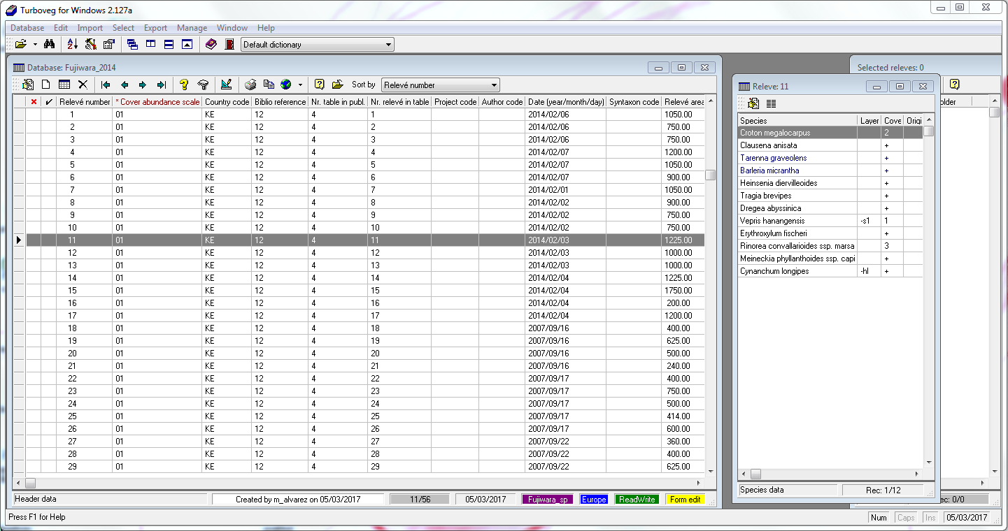
In the case there is an error message produced by inconsistent data structure, there is the possibility of importing the data as a list for further inspection.
Fujiwara_list <- tv2vegtable("Fujiwara_2014", tv_home, output="list")
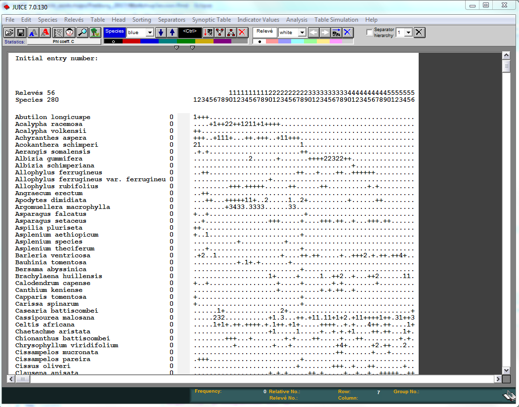
Export to Juice
Export of data for Juice follows a similar procedure as for cross tables.
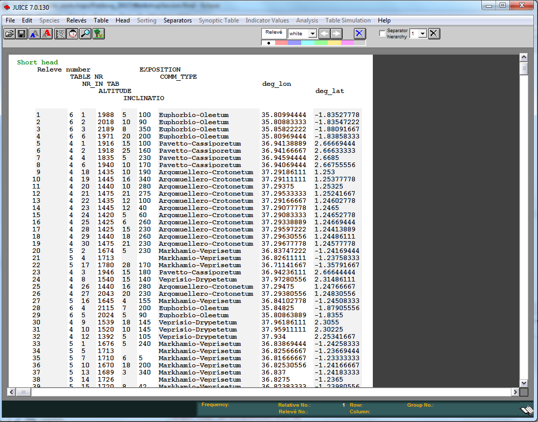
write_juice(Fujiwara, "RiftValley",
  COVER_CODE ~ ReleveID + AcceptedName + LAYER,
  header=c("TABLE_NR","NR_IN_TAB","ALTITUDE","INCLINATIO","EXPOSITION",
    "COMM_TYPE"),
  FUN=paste0)
Besides the vegtable object, the most important elements
to export are:
formulaindicating how to construct the cross table.headerto show which variables should be exported for the head data.coordswith the names of coordinates, if present.FUNthe function used for aggregate multiple records.
The values for coords should be as decimal degrees and
in the spatial system WGS 84. In Juice such information
will be included in the header data as columns deg_lon
and deg_lat, allowing the display of plots in
Google Earth. The previous command has generated two
files, namely RiftValley_table.txt and
RiftValley_header.txt.
For importing the table, you may follow the steps:
- Open Juice
- In menu
File -> Import -> Table -> From Spreadsheet File (e.g. EXCEL Table) - Browse to RiftValley_table.txt and
Open - In the last step, select the option
Braun-Blanquet CodesandFinish - Finally, save the new file
Now for the head:
- In menu
File -> Import -> Header Data -> From Comma Delimited File - Browse to RiftValley_header.txt and
Open
Map in leaflet
For geo-referenced plots, you can easily map the location of the
plots, for instance using the package leaflet.
Then, hopefully you enjoyed the session and did not get too much error messages.
Updated on
20-06-2022
Aknowledgements
This workshop was supported by the project GlobE-wetlands.