Installation
Both packages taxlist and
vegtable
are released in the Comprehensive R Archive Network
(CRAN). Since taxlist is a dependency of
vegtable, both will be installed in the following
command:
install.packages("vegtable", dependencies = TRUE)
Alternatively, you can install the development versions from their repositories at GitHub.
library(devtools)
install_github("ropensci/taxlist", build_vignettes = TRUE)
install_github("kamapu/vegtable")
An additional package including some example data required for this session have also to be installed from GitHub.
install_github("kamapu/sanmartin1998")
Working with species lists only
Before starting with the work, do not forget to load the installed packages into your R-session:
In this first section we focus on the taxlist objects,
which are specialized for handling taxonomic lists. For more details on
the theory behind this package, see Alvarez and Luebert (2018).
The package taxlist includes a own data set called
Easplist.
Easplist
object size: 761.4 Kb
validation of 'taxlist' object: TRUE
number of taxon usage names: 5393
number of taxon concepts: 3887
trait entries: 311
number of trait variables: 1
taxon views: 3
concepts with parents: 3698
concepts with children: 1343
hierarchical levels: form < variety < subspecies < species < complex < genus < family
number of concepts in level form: 2
number of concepts in level variety: 95
number of concepts in level subspecies: 71
number of concepts in level species: 2521
number of concepts in level complex: 1
number of concepts in level genus: 1011
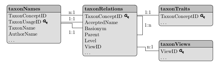
number of concepts in level family: 186The information stored in a taxlist object is organized
in four column-oriented tables following a relational model and
allocated in own slots within the object. The access to the respective
slots in R is done with the symbol @ or alternatively using
the function slot().
head(Easplist@taxonNames)
  TaxonUsageID TaxonConceptID              TaxonName
1            1              1 Abelmoschus esculentus
2        52313              1    Hibiscus esculentus
3            2              2       Abutilon indicum
4            3              3   Abutilon mauritianum
5        50361              3         Pavonia patens
6            4              4   Acacia drepanolobium
            AuthorName
1          (L.) Moench
2                   L.
3                 (L.)
4       (Jacq.) Medik.
5     (Andrews) Chiov.
6 Harms ex Y. Sjöstedthead(Easplist@taxonRelations)
  TaxonConceptID AcceptedName Basionym Parent   Level ViewID
1              1            1       NA  54753 species      1
2              2            2       NA  54754 species      1
3              3            3       NA  54754 species      1
4              4            4       NA  54755 species      1
5              5            5       NA  54755 species      1
6 6 6 NA 54755 species 1head(Easplist@taxonTraits)
  TaxonConceptID          life_form
1              7       phanerophyte
2              9       phanerophyte
3             18 facultative_annual
4             20 facultative_annual
5             21    obligate_annual
6 22 chamaephytehead(Easplist@taxonViews)
  ViewID                                 secundum view_bibtexkey
1      1            African Plant Database (2012)  CJBGSANBI2012
2      2 Taxonomic Name Resolution Service (2018)       TNRS2018
3      3                    The Plant List (2013)        TPL2013
Summaries
The function summary() can be used to query information
of a taxon or a set of taxa.
summary(Easplist, ConceptID = "Typha domingensis", secundum = "secundum",
    exact = TRUE)
------------------------------
concept ID: 50105
view ID: 1 - African Plant Database (2012)
level: species
parent: 55040 Typha L.

# accepted name:
50105 Typha domingensis Pers.

# synonyms (9):
51999 Typha australis Schumach.
53124 Typha angustifolia ssp. australis (Schumach.) Graebn.
53125 Typha aequalis Schnizl.
53126 Typha angustata Bory & Chaub.
53127 Typha angustifolia ssp. angustata (Bory & Chaub.) Briq.
53128 Typha angustata var. abyssinica Graebn.
53129 Typha angustata var. aethiopica Rohrb.
53130 Typha aethiopica (Rohrb.) Kronfeldt
53131 Typha schimperi Rohrb.
------------------------------
In this command line the parameter ConceptID is used to
query a taxon name. The parameter secundum is set to the
name of a column in slot taxonViews that will be
appended to the taxon view ID, which may not be informative alone. The
setting exact = TRUE indicates that the queried name have
to be a perfect match to the taxon usage names in the data set,
otherwise sub-specific taxa of the queried species may be also
retrieved. The command retrieves the ID of the queried taxon, the ID of
the taxon view (for a
definition see Alvarez
and Luebert, 2018), the taxonomic rank, the ID and name of
the parent taxon (if suitable), the accepted name and a listing of
synonyms.
Note in the display that the taxon concept ID and the ID of the parent refer to their taxon concept IDs, which is the primary key at slot taxonRelations, while the IDs in front of the accepted name and synonyms refer to the IDs of the respective taxon usage names, which is the primary key at slot taxonNames.
You can also display an indented list with the following command.
indented_list(Easplist, "Typha")
Typhaceae
 Typha L.
   Typha capensis (Rohrb.) N.E. Br.
   Typha latifolia L.
   Typha domingensis Pers.
The function print_name() can be used to format
scientific names when writing rmarkdown documents. The
following example is adapted from the documentation of the function.
Note in the example that the option style = "expression" is
meant to be used in plot devices.
## Accepted name with author
print_name(Easplist, 363, style = "expression")
expression(italic("Ludwigia adscendens") ~ "ssp." ~ italic("diffusa")~"(Forssk.) P.H. Raven")## Including taxon view
print_name(Easplist, 363, style = "expression", secundum = "secundum")
expression(italic("Ludwigia adscendens") ~ "ssp." ~ italic("diffusa")~"(Forssk.) P.H. Raven"~"sec. African Plant Database (2012)")## Second mention in text
print_name(Easplist, 363, style = "expression", second_mention = TRUE)
expression(italic("L. adscendens") ~ "ssp." ~ italic("diffusa")~"(Forssk.) P.H. Raven")## Using name ID
print_name(Easplist, 50037, style = "expression", concept = FALSE)
expression(italic("Ludwigia stolonifera")~"(Guill. & Perr.) P.H. Raven")## Markdown style
print_name(Easplist, 363, style = "markdown")
[1] "*Ludwigia adscendens* ssp. *diffusa* (Forssk.) P.H. Raven"## HTML style
print_name(Easplist, 363, style = "html")
[1] "<i>Ludwigia adscendens</i> ssp. <i>diffusa</i> (Forssk.) P.H. Raven"## LaTeX style for knitr
print_name(Easplist, 363, style = "knitr")
[1] "\\textit{Ludwigia adscendens} ssp. \\textit{diffusa} (Forssk.) P.H. Raven"Working with vegetation-plots
Further examples will be applied to a data set available at the
installed package sanmartin1998, which corresponds to plot
observations in grasslands and semi-aquatic communities from Temuco,
Chile. This data set was originally published by San Martín et al. (1998) and is
stored in the database sudamerica (https://kamapu.github.io/sudamerica/, see also
Alvarez et al.,
2012).
releves
## Metadata
   db_name: sudamerica
   description: Database for vegetation-plots from South America.
   taxonomy: sam_splist
   bibtexkey: NA
   object size: 195.8 Kb
   validity: TRUE

## Content
   number of plots: 80
   plots with records: 80
   variables in header: 13
   number of relations: 2

## Taxonomic List
   taxon names: 548
   taxon concepts: 199
   validity: TRUE
Structure
Objects of class vegtable are structured into 8 slots,
where the slots species, header, and
samples are the essential ones.
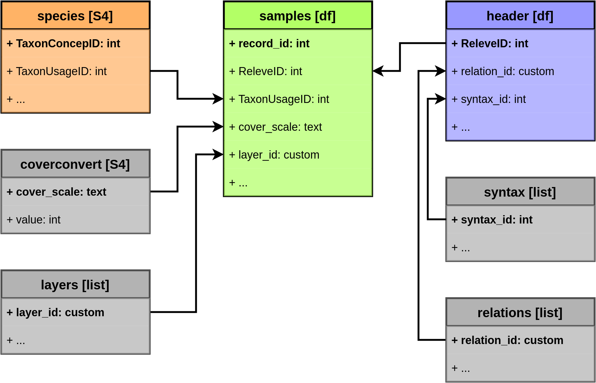
The taxonomic list is handled as a taxlist object and is
located at the slot species:
summary(releves@species)
object size: 98 Kb
validation of 'taxlist' object: TRUE

number of taxon usage names: 548
number of taxon concepts: 199
trait entries: 85
number of trait variables: 8
taxon views: 10

concepts with parents: 164
concepts with children: 113

hierarchical levels: form < variety < subspecies < species < section < subgenus < genus < subfamily < family < phylum
number of concepts in level form: 0
number of concepts in level variety: 6
number of concepts in level subspecies: 1
number of concepts in level species: 86
number of concepts in level section: 0
number of concepts in level subgenus: 0
number of concepts in level genus: 71
number of concepts in level subfamily: 0
number of concepts in level family: 35
number of concepts in level phylum: 0
The slot header is simply a data frame including information related to single plot observations, for instance size of the plot, record date, results of soil analyses, etc.
head(releves@header)
    ReleveID table_number column_number plot_size plot_length
445     6091            3             1        25          NA
469     6115            3             2        25          NA
470     6116            3            13        25          NA
592     6234            2             8        25          NA
593     6235            2            10        25          NA
594     6236            2            11        25          NA
    plot_width elevation community_type page_number    db_name
445         NA       163            565         105 sudamerica
469         NA       163            565         105 sudamerica
470         NA       199            565         105 sudamerica
592         NA       199            534         104 sudamerica
593         NA        77            534         104 sudamerica
594         NA       168            534         104 sudamerica
    data_source longitude latitude
445          29  -72.7201 -38.6727
469          29  -72.7201 -38.6727
470          29  -72.7341 -38.6310
592          29  -72.7341 -38.6310
593          29  -72.7440 -38.6846
594          29  -72.6958 -38.7141
Records of species in plots are stored in slot samples. Against the commonly used cross tables (species by plots or plots by species), this slot is organized in columns (column-oriented table, a.k.a database list).
head(releves@samples)
      record_id ReleveID TaxonUsageID cover_percentage
10575    138697     7285        20972             15.0
10576    138698     7285        23744             60.0
10577    138699     7285         9373             20.0
10578    138700     7285       196060              0.5
10579    138701     7285        35072              5.0
10580    138702     7285         9953              0.5
The slot coverconvert have an own, homonymous class
and is used as container for cover conversion tables. These tables can
be used for conversion of cover codes, which will be done by the
function transform(). The example on releves does not
include cover conversion tables but the data set installed with
vegtable does it.
summary(Kenya_veg@coverconvert)
## Number of cover scales: 3

* scale 'br_bl':
  Levels    Range
1      r    0 - 1
2      +    0 - 1
3      1    1 - 5
4      2   5 - 25
5      3  25 - 50
6      4  50 - 75
7      5 75 - 100

* scale 'b_bbds':
  Levels    Range
1      r    0 - 1
2      +    0 - 1
3      1    1 - 5
4     2m    1 - 5
5     2a   5 - 15
6     2b  15 - 25
7      3  25 - 50
8      4  50 - 75
9      5 75 - 100

* scale 'ordin.':
  Levels    Range
1      1    0 - 1
2      2    0 - 1
3      3    1 - 5
4      4    1 - 5
5      5   5 - 15
6      6  15 - 25
7      7  25 - 50
8      8  50 - 75
9      9 75 - 100
The slot relations is a list of data frames that provide additional information for classes of categorical variables stored in slot header. These tables correspond to pop-up tables of Turboveg 2.
names(releves@relations)
[1] "community_type" "data_source" head(releves@relations$community_type)
  community_type
1            298
2            305
3            307
4            310
5            313
6            315
                                                       community_name
1            Loudetia phragmitoides-Hyparrhenia bracteata-communities
2                                             Loudetio-Fimbristyletum
3                                            Euphorbieto-Portulacetum
4                                 Amaranthus sp- Synedrella nodiflora
5                               Pennisetum purpureum-Acalypha ciliata
6 Sporobolus festivus-Hysanthes trichotoma (sous-association typique)
While in the header table such categorical variables may be cryptic,
there is an option to insert columns from relations into header by using
relation2header(). By this way, yo do not only see a
community id, which is just a number, but you can also see the
respective names of the plant communities that correspond to the syntaxa
assigned to the plots originally by the publication.
releves <- relation2header(releves, "community_type")
head(releves@header)
    ReleveID table_number column_number plot_size plot_length
445     6091            3             1        25          NA
469     6115            3             2        25          NA
470     6116            3            13        25          NA
592     6234            2             8        25          NA
593     6235            2            10        25          NA
594     6236            2            11        25          NA
    plot_width elevation community_type page_number    db_name
445         NA       163            565         105 sudamerica
469         NA       163            565         105 sudamerica
470         NA       199            565         105 sudamerica
592         NA       199            534         104 sudamerica
593         NA        77            534         104 sudamerica
594         NA       168            534         104 sudamerica
    data_source longitude latitude
445          29  -72.7201 -38.6727
469          29  -72.7201 -38.6727
470          29  -72.7341 -38.6310
592          29  -72.7341 -38.6310
593          29  -72.7440 -38.6846
594          29  -72.6958 -38.7141
                            community_name
445 Mentho pulegium-Agrostietum capillaris
469 Mentho pulegium-Agrostietum capillaris
470 Mentho pulegium-Agrostietum capillaris
592                       Juncetum proceri
593                       Juncetum proceri
594                       Juncetum proceri
Statistics
The packages vegtable and taxlist are
rather specialized on data manipulation than on data analysis.
Nevertheless some common descriptive statistics and summaries that can
be used for further statistical analyses are implemented.
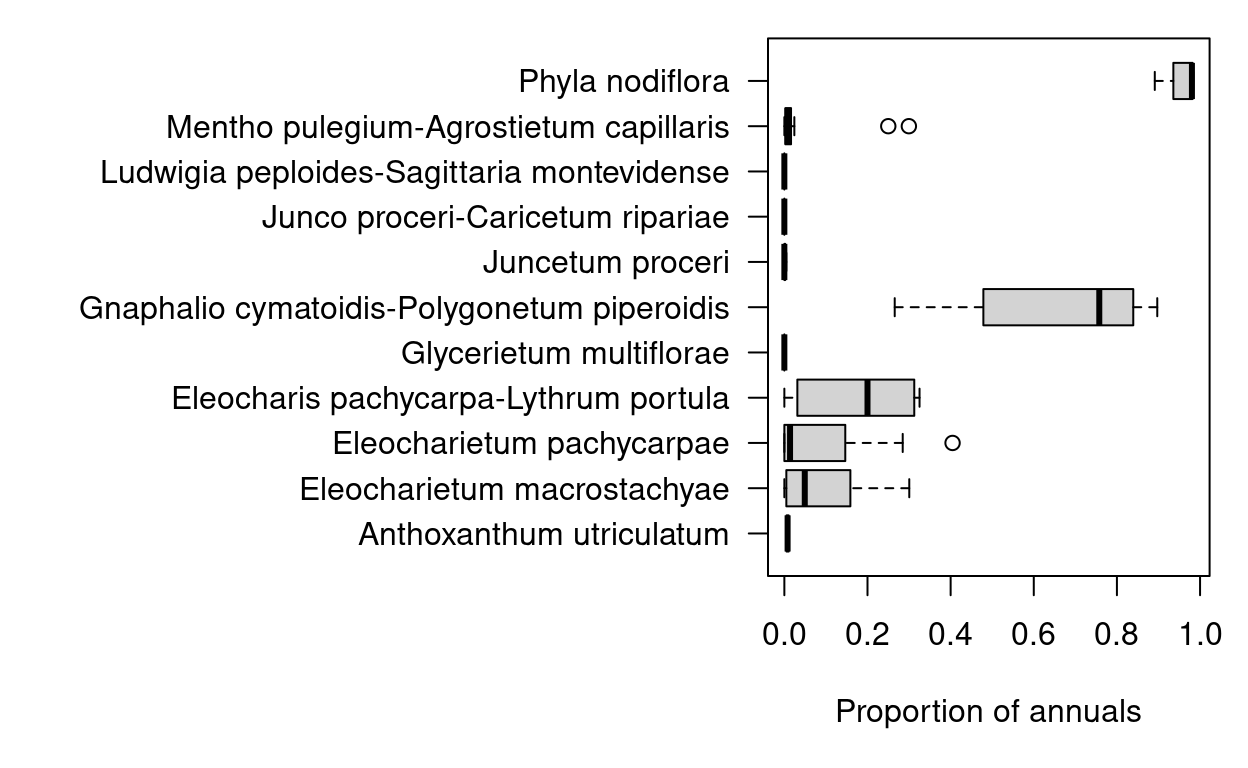
Trait proportions
In this data set, for instance, life forms are inserted as attributes
of the recorded species. Since this attribute is a categorical variable,
summaries at the plot level can only be done as proportions. The
function trait_proportion() is suitable for such kind of
summaries. Note that the best way to collect statistics calculated for
plots is adding them as new columns into the slot
header, which is done by the option
in_header=TRUE. Additionally, the option
weight="cover_percentage" is indicating that the cover
percentage stored in the slot samples will be used as
weight for the respective life from classes.
releves <- trait_proportion(trait="life_form", object=releves,
    head_var="ReleveID", include_nas=FALSE, weight="cover_percentage",
    in_header=TRUE)
By default, the function added at slot header one
column per level in the traits variable appending a suffix (default
_prop). Just to remind you, we used the function
relation2header() in order to add the names of the recorded
communities in the slot header.
# Add community names to the header table
releves <- relation2header(releves, relation="community_type")

# Display mean values per plant communities
aggregate(annual_prop ~ community_name, data=releves@header, FUN=mean)
                                community_name annual_prop
1                     Anthoxanthum utriculatum 0.007826989
2                  Eleocharietum macrostachyae 0.096678841
3                    Eleocharietum pachycarpae 0.092635324
4        Eleocharis pachycarpa-Lythrum portula 0.173790650
5                      Glycerietum multiflorae 0.000000000
6  Gnaphalio cymatoidis-Polygonetum piperoidis 0.650889962
7                             Juncetum proceri 0.001167405
8             Junco proceri-Caricetum ripariae 0.000000000
9   Ludwigia peploides-Sagittaria montevidense 0.000000000
10      Mentho pulegium-Agrostietum capillaris 0.041020366
11                             Phyla nodiflora 0.958893907
# The same information as boxplot
par(mar=c(5, 20, 1, 1), las=1)
boxplot(annual_prop ~ community_name, data=releves@header, horizontal=TRUE,
xlab="Proportion of annuals", ylab="")
Before you continue, note that the first argument in the function is
a formula indicating on the left a response as left term
(in this case the statistic describing a categorical trait variable) and
the factors as right terms (grouping variables for the plots). This kind
of objects will be frequently used in functions dealing with
vegtable objects.
Trait Statistics
For numerical taxonomic traits statistical parameters such as
averages and standard deviation can be calculated per plot. For instance
the data set releves is also including Ellenberg’s
indicator values (see
Ellenberg et
al., 2001), which were collected from Ramírez et al. (1991) and San Martín et al.
(2003).
The calculation of trait statistics is done by the function
trait_stats(). In the parameter FUN we can use
a statistical function such as mean() but we can also
define an statistic using the cover values as weights for the
calculation. In this case we can calculate weighted means:
\[\bar{x} = \frac{\sum{x_{i} \cdot w_{i}}}{\sum{w_{i}}}\]
Here \(\bar{x}\) is the mean indicator figure for a plot, \(x_{i}\) is the indicator value of the ith species in this plot, and \(w_{i}\) is the weight of the same species (cover value) in the plot. In R we define it as a function:
In the function trait_stats() we can query indicator
figures through a formula. Note that this formula may include multiple
variables on the left terms for the simultaneous calculation of
indicator values.
releves <- trait_stats(ind_n + ind_h ~ ReleveID, releves,
    FUN=weighted_mean,  include_nas=FALSE, weight="cover_percentage",
    suffix="_wmean", in_header=TRUE)
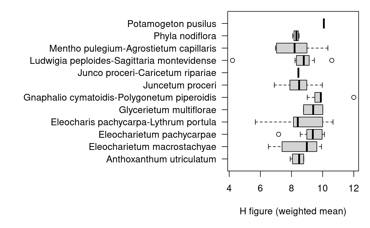
The resulting values may be useful to compare different plant communities or to test relationships between different variables, for instance an expected correlation between the humidity indicator and the proportion of annuals.
par(mar=c(5, 20, 1, 1), las=1)
boxplot(ind_h_wmean ~ community_name, data=releves@header, horizontal=TRUE,
    xlab="H figure (weighted mean)", ylab="")
# Linear regression model
Mod <- lm(annual_prop ~ ind_h_wmean, data=releves@header)

# plot
plot(releves@header[,c("ind_h_wmean", "annual_prop")], xlab="H figure",
    ylab="Proportion of annuals", pch=20, col="darkgrey")
abline(Mod, lty=2, col="red")
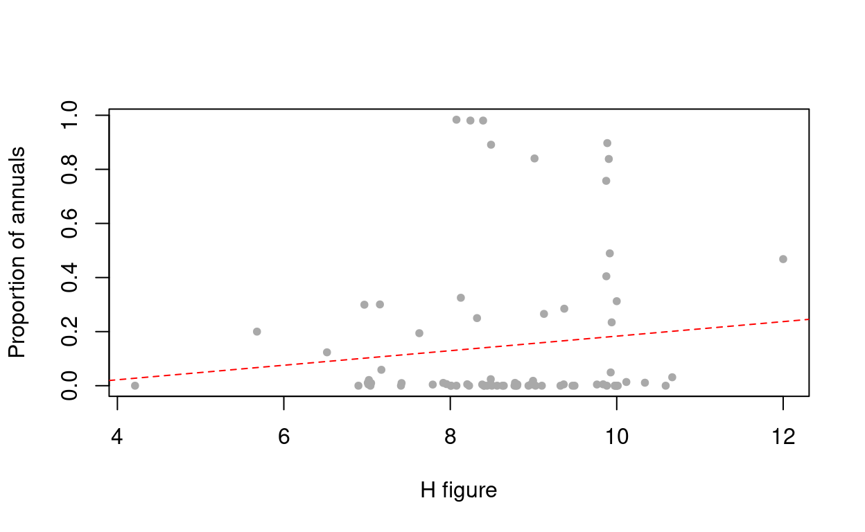
Well, it is not a nice distribution of observations but still suggesting a negative tendency in the proportion of annuals by increasing humidity indicator, as expected.
Statistics from taxonomic information
Taxonomic information (taxonomic ranks and parent-child
relationships) are not directly available for statistical descriptions
in taxlist objects. If we need to calculate proportions of
determined genera or families in the plots, we can pass the taxonomy to
the taxon traits table with the function tax2traits(). You
need to set get_names=TRUE, otherwise only taxon IDs
(numbers) will be inserted in the traits table.
releves@species <- tax2traits(releves@species, get_names=TRUE)
head(releves@species@taxonTraits)
   TaxonConceptID origin_status life_form ind_l ind_t ind_r ind_n
2           57184        native perennial    NA    NA    NA    NA
10          57504        native perennial     6     5     4     3
17          58062        native perennial    NA    NA    NA    NA
41          61842          <NA>      <NA>     8     6     5     7
43          61852          <NA>      <NA>     6     7    NA     8
44          61853     adventive perennial     8     5     5     5
   ind_h ind_s variety subspecies                species
2     NA    NA    <NA>       <NA>      Adesmia corymbosa
10     6    NA    <NA>       <NA>      Dichondra sericea
17    NA    NA    <NA>       <NA>     Setaria parviflora
41    12    NA    <NA>       <NA>  Callitriche palustris
43     5    NA    <NA>       <NA> Echinochloa crus-galli
44     5    NA    <NA>       <NA>  Arrhenatherum elatius
           genus         family
2        Adesmia    Leguminosae
10     Dichondra Convolvulaceae
17       Setaria        Poaceae
41   Callitriche Plantaginaceae
43   Echinochloa        Poaceae
44 Arrhenatherum        Poaceae
Now we can compare, for instance, the proportion of species belonging to the family Poaceae (grasses) in the different plant communities.
releves <- trait_proportion("family", releves, head_var="ReleveID",
    trait_level="Poaceae", include_nas=FALSE, weight="cover_percentage",
    in_header=TRUE)

# Compare communities by proportion of Poaceae
par(mar=c(5, 20, 1, 1), las=1)
boxplot(Poaceae_prop ~ community_name, data=releves@header,
    horizontal=TRUE, xlab="Proportion of Poaceae", ylab="")
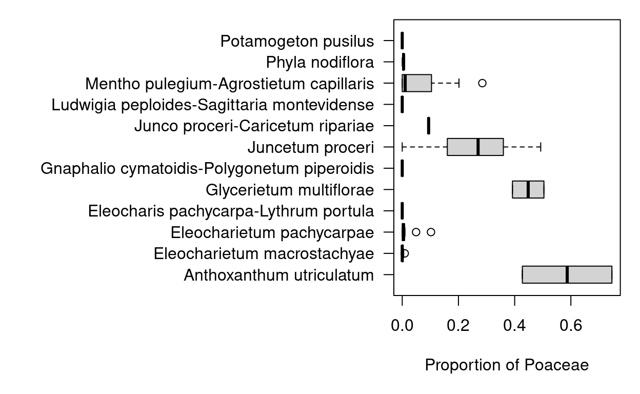
This graphic is advising us that maybe few of these communities can be considered as grasslands sensu stricto.
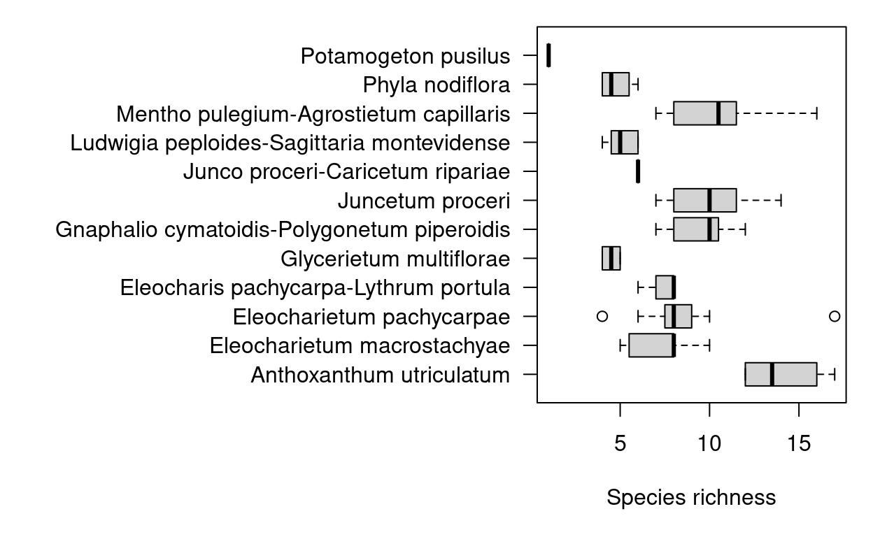
The function count_taxa() is defined for calculation of
number of taxa at specific taxonomic ranks. Note that this function may
be smart enough to aggregate taxa into the corresponding ranks, for
instance the calculation of species numbers may also include
sub-specific taxa in their respective species (option
include_lower=TRUE).
releves <- count_taxa(species ~ ReleveID, releves, include_lower=TRUE,
    in_header=TRUE)

# Compare communities by species richness
par(mar=c(5, 20, 1, 1), las=1)
boxplot(species_count ~ community_name, data=releves@header,
    horizontal=TRUE, xlab="Species richness", ylab="")
Cross tables and Maps
Most of the applications used for floristic comparisons require data
in form of a cross table. Furthermore, species composition of
communities may be more evident by displaying data, for instance, in a
table of species by plots. To arrange data in such a way we can apply
the function crosstable().
In order to reduce the data set, we will apply the function
subset(), selecting plots of the association Juncetum
proceri.
## Metadata
   db_name: sudamerica
   description: Database for vegetation-plots from South America.
   taxonomy: sam_splist
   bibtexkey: NA
   object size: 217.2 Kb
   validity: TRUE

## Content
   number of plots: 15
   plots with records: 15
   variables in header: 20
   number of relations: 2

## Taxonomic List
   taxon names: 548
   taxon concepts: 199
   validity: TRUE
In the function crosstable() we indicate as formula in
the left term the numeric variable used to fill the table, the first
right term is the group variable used for the columns and the further
right terms are group variables defining the rows of the cross table.
Note that the taxa in the formula can be addressed by either one of two
keywords, namely TaxonName for the use of original
entry names (taxon usage names) or AcceptedName for use
of the respective names considered as accepted in slot species. We also
set the arguments FUN=max defining the function used to
merge multiple occurrences of a taxon in a plot and
na_to_zero=TRUE to fill absence.
juncetum_cross <- crosstable(cover_percentage ~ ReleveID + AcceptedName,
    data=juncetum, FUN=max, na_to_zero=TRUE)
head(juncetum_cross)
                         AcceptedName 6236 6237 6239 7285 7423 7643
1    Adesmia corymbosa var. corymbosa  0.5  0.5  0.5   10  0.5  0.5
2                 Agrostis capillaris 10.0 30.0  0.0   15 40.0 20.0
3            Anthoxanthum utriculatum  0.0  0.0  0.0    0  0.0  0.0
4 Arrhenatherum elatius var. bulbosum  0.0  0.0  0.0    0  0.0  0.0
5                Baccharis sagittalis  0.0  0.0  0.0    0  0.0  0.0
6               Centipeda elatinoides  0.0  0.5  0.0    0  0.0  0.5
  6234 6235 6238 6588 6589 6804 6805 7294 7303
1    0  0.0  0.0    0    0  0.0    0    0    0
2   50 20.0 40.0   10   30 20.0   50   20   50
3    0  0.5  0.0    0    0  0.0    0    0    0
4    0  0.5  0.0    0    0  0.0    0    0    0
5    0  0.0  0.5    0    0  0.0    0    0    0
6    0  0.0  0.0    0    0  0.5    0    0    0
When plots are geo-referenced, you can show their locations using the
package leaflet.
Updated on
24-06-2022
Acknowledgement
The data sets and routines demonstrated here have been previously tested by Elena Gómez in the context of her thesis for the degree of MSc. (Gómez, 2020). Any further comments and suggestions are kindly welcomed.